Notas técnicas
MCM Alchimia Methods: solved examples on computer-aided uncertainty quantification
Metodología de MCM Alchimia: ejemplos resueltos de estimación de incertidumbre asistida por computadora
Metodologia MCM Alchimia: exemplos resolvidos de quantificação de incerteza auxiliada por computador
 Pablo Constantino pconstan@latu.org.uy
MCM Alchimia Methods: solved examples on computer-aided uncertainty quantification
INNOTEC, núm. 22, e547, 2021
Laboratorio Tecnológico del Uruguay

Esta obra está bajo una Licencia Creative Commons Atribución-NoComercial 4.0 Internacional.
Recepción: 15 Julio 2020
Aprobación: 22 Abril 2021
Abstract: MCM Alchimia is a free and multilingual desktop application, which runs on Windows. It is available to download from the Internet. This application implements the processes indicated in the Guide to the Expression of Uncertainty in Measurement (GUM) and the Supplement 1 of this document, easily obtaining measurement results and associated expanded uncertainty, with a detailed uncertainty budget according to GUM, and a summary of statistical parameters of the simulated sample obtained by Monte Carlo Method (MCM). This work establishes an intuitive and rapid guide for estimating measurement uncertainties by GUM and MCM methods with the software MCM Alchimia, through discussion of five examples from document JCGM 100: 2008 and three from JCGM 101: 2008. Some features and algorithms of the software are explained in detail. Particularly, functions and tools that are not available in other similar software applications, for example, the estimation of uncertainties in test models that involve the use of least-square fittings. In addition, more intuitive approaches to some problem than those suggested in the JCGM guides are shown, discussing different features available in the software to perform an easy data treatment of complex measurement models.
Keywords: GUM, MCM, Monte Carlo, JCGM 100 examples.
Resumen: MCM Alchimia es una aplicación de escritorio multilingüe y gratuita para Windows, que está disponible para descargar de Internet. Esta aplicación implementa los procesos indicados en la Guía para la Expresión de la Incertidumbre de Medida (GUM) y el Suplemento 1 de este documento, obteniendo rápidamente resultados de medición e incertidumbre expandida asociada, con un detallado presupuesto de incertidumbre según GUM y un resumen de parámetros estadísticos de la muestra obtenida por simulación de Monte Carlo (MCM). Este trabajo establece una guía intuitiva y rápida para estimar las incertidumbres de medición, utilizando el software MCM Alchimia, a través del análisis de la solución por GUM y MCM de cinco ejemplos del documento JCGM 100: 2008 y tres de JCGM 101: 2008. Se explican pormenorizadamente algunos aspectos y algoritmos del software, deteniéndose en funciones y herramientas que no se encuentran en otras aplicaciones de software similares, por ejemplo, la estimación de incertidumbres en modelos de ensayo que implican el uso de curvas obtenidas por ajuste de mínimos cuadrados. Además, se muestran enfoques más intuitivos para la solución usando MCM Alchimia que los sugeridos en las guías JCGM, discutiendo diferentes características disponibles en el software que permiten realizar un tratamiento de datos rápido de modelos matemáticos complejos.
Palabras clave: GUM, MCM, Monte Carlo, ejemplos JCGM 100.
Resumo: MCM Alchimia é um software de desktop multilíngue gratuito que roda em Windows. Ele está disponível para baixar da Internet. Esta aplicação implementa os processos indicados na Guia para a Expressão de Incerteza na Medição (GUM) e no Suplemento 1 deste documento, obtendo facilmente resultados de medição e incerteza expandida associada, com um quadro de incerteza detalhado de acordo com GUM, e um resumo estatístico de parâmetros da amostra simulada obtida pelo Método de Monte Carlo (MCM). Este trabalho estabelece um guia intuitivo e rápido para estimar incertezas de medição pelos métodos GUM e MCM com o software MCM Alchimia, por meio da discussão de cinco exemplos do documento JCGM 100: 2008 e três do JCGM 101: 2008. Alguns recursos e algoritmos do software são explicado em detalhes. Particularmente, funções e ferramentas que não estão disponíveis em outros aplicativos de software semelhantes, por exemplo, a estimativa de incertezas em modelos de teste que envolvem o uso de ajustes mínimos quadrados. Além disso, são mostradas para algum problema abordagens mais intuitivas do que as sugeridas nos guias JCGM, discutindo os diferentes recursos disponíveis no software para realizar um tratamento de dados fácil de modelos de medição complexos.
Palavras-chave: GUM, MCM, Monte Carlo, JCGM 100 exemplos.
INTRODUCTION
MCM Alchimia (Alchimia Project, s.d.) is a desktop application that automates the process of evaluating the uncertainty associated to the results of an output quantity or measurand which can be obtained directly from the combination of an unlimited number of input quantities, whose value, uncertainty and probability distribution functions (hereinafter PDF) are known. The software estimates the measurement uncertainty according to the general directives established in the guide JCGM 100:2008 (BIPM, et al., 2008a), as well as through the Monte Carlo method, established in supplement 1 of this same guide: JCGM 101:2008 (BIPM, et al., 2008b). Input quantities can be correlated or not, or even be the result of an interpolation from a calibration curve. The first approach (hereinafter GUM, an acronym for the words Guide of Uncertainty of Measurement that the aforementioned document references), establishes an approximate estimation method represented by the Uncertainty Propagation Law, an equation based on the development of the measurand function in first order Taylor series. The Monte Carlo approach (hereinafter MCM, acronym for Monte Carlo Method) is based on the propagation of distributions from a random sampling in probability distribution functions. This work does not delve into the general aspects of these methods or their differences, but rather it offers a simple software alternative that implements both methods to solve specific situations.
Motivation and milestones in development. MCM Alchimia (Alchimia Project, s.d.) was developed in 2012 in an attempt to provide metrologists, laboratory analysts and researchers with a simple tool for estimating uncertainties by the Monte Carlo method. Most of the software tools that performed the estimation of uncertainties available at the time, did so by means of the law of propagation of uncertainties or GUM. Alternatively, existing applications that performed Monte Carlo simulations were rather either focused on the generality of the method or problem resolution in mathematics and economics. Technicians who carry out measurements handle more information than the characteristics of the sample resulting from the simulation, for example the contribution of uncertainty of the input quantities. The essential computer aspects and minimum statistical requirements for a software application that performs the estimation of uncertainties by MCM were studied, in order to ensure that the estimation of uncertainty, even in complex mathematical models, yields results that are valid according to the ISO GUM (Constantino, 2013). Based on these studies, the first version of the application is created, and one year after, a second version is released containing improvements to the interface and to simulation algorithms.
In 2016, aiming particular needs in chemical measurements, a specific module was developed to perform Monte Carlo simulations in measurement models that included interpolation values in an external calibration curve as input quantities. In its final version, this module is able to obtain adjustment curves for ordinary, inverse and total least squares, in the latter case, by means of the method called Primary Component Analysis (PCA). The input data for the curve can be constant or have uncertainties. Uncertainties can be assigned to both the independent and dependent variable values. The uncertainty for these input quantities is individual for each pair of data, and can be assigned Gaussian, rectangular, or triangular probability distribution functions, as well as constants, that is, without uncertainty. From this curve, interpolated magnitudes on both axis can be included in the test model or, otherwise, directly use regression parameters slope, intercept or even the standard error of the regression as a component of uncertainty. This module was included in version 3 of MCM Alchimia (Alchimia Project, s.d.), and is, to this day, the only free software application that performs uncertainty analysis on calibration curves by the Monte Carlo method. The operation of the regression module is detailed in Example 2 of this document.
In 2018, version 4 was launched, adding an estimation module to perform calculations according to the classic GUM framework. This module yield an uncertainty budget table with estimated variances of each particular contribution, degrees of freedom, effective degrees of freedom product of the Welch-Sattertwhite formulae, and the correct expression of measurement and associated uncertainty, according to ISO GUM JCGM 100:2008 (BIPM, et al., 2008a). Finally, in the year 2020 a new revision, version 5 of this software is carried out, adding advanced specifications of reliability and degrees of freedom for the input parameters with contributions of type B uncertainty, and regression analysis by GUM framework as the main improvements.
In the following sections, the particularities of the application and the calculation methods used are studied in detail, subjecting these aspects to the resolution of the examples documented in the reference standards.
METHODS
To establish a working method with the MCM Alchimia software (Alchimia Project, s.d.), most of the examples contained in GUM and its supplement 1 are thoroughly studied, proposing the use of different calculation strategies, if they exist, or even some features of the software that facilitates the work of quantifying uncertainty. In addition, the differences found between the results obtained by GUM and MCM are discussed. Although the application is very intuitive and contains almost no configuration menus, the calculation approach that best represents the case under study is not always obvious. The examples detailed below are not fully developed, as they appear in the reference document, only the computer-aided solution using MCM Alchimia is discussed (Alchimia Project, s.d.), as well as the aspects and features of the application that will improve or simplify obtaining results. The main aspect to study in each example will be described under its title.
The objective that is sought with this technical note is to provide a method as easy as possible so that the examples can be resolved with the chosen software and as it is setted out in the reference documents. For this, the units in tables and calculations were kept exactly as indicated in the original documents, warning the reader that not all examples are raised and resolved in international system units (SI).
On the other hand, regarding the chosen software, it is possible that some terms are not consistent with the VIM (International Vocabulary of Metrology) – JCGM 200:2012 (BIPM, et al., 2012). In particular, it is relevant to warn that the term Confidence Interval should be understood as Coverage Interval.
Example 1. Calibration of end gauge blocks (from: JCGM 100:2008, H1)
Topic: Calculation strategy and workflow
The measurement objective is to obtain the calibration error with respect to the nominal value. This error is obtained by mechanical comparison, with a comparator equipment, from the difference in length between the block under test and a calibrated standard block. The mathematical model used for this test according to the reference document, and which can be typed directly in the equation field of the step 2 of the application would be:

Equation 1
Where l is the length at 20 °C of sample gauge block, ls the length of standard block at 20 °C from its calibration certificate, δθ y δα correspond respectively to the difference between test temperatures and between the coefficients of thermal expansion for the standard block and the block under test. αS is the coefficient of thermal expansion of the standard block, while θ represents the temperature deviation of the standard block. It should be noted in the statement that some magnitudes of the model include more than one source of uncertainty. For example, the difference between the blocks (.), whose value is the mean of the observations, presents an uncertainty component due to repeatability (drep). Adding to that, in this example, is assigned a historical value (pooled standard deviation), another due to random effects of the comparator (drnd) and a third due to the systematic effects of the comparator (dsist). In the same way, θ includes uncertainties components for the average temperature of the calibration bench (θtb) and by the cyclical variation of the laboratory temperature (θcyc).
It is common for all test models to have quantities with more than one source of uncertainty. The recommended proceeding when implementing these models in MCM Alchimia (Alchimia Project, s.d.), is to split these magnitudes previously into a constant with their value and add their uncertainty components with value equals zero. In this and the following examples, it will be done in this way. Therefore, equation 1 split down into sources of uncertainty will be:

Equation 2
u(xi) and degrees of freedom for dsist, δα y δθ are affected by the concept of reliability, according to what is stated in the document. As usual for a standard uncertainty obtained from a Type B evaluation, most available software assigns infinite degrees of freedom. However, the JCGM 100 (BIPM, et al., 2008a) guide establishes an equation to calculate this value.

Equation 3
Equation 3, G.3 in JCGM 100:2008 (BIPM, et al., 2008a) defines degrees of freedom (vi) for the type B evaluation of a standard uncertainty with a reliability based on available information. The 5th version of MCM Alchimia (Alchimia Project, s.d.) implements this equation and, therefore, the possibility of working with reliability values in the most common PDF, Gaussian (Normal) and Rectangular functions. In these cases, these distributions can be used in the same way as in previous versions, with infinite degrees of freedom, or a finite number of degrees of freedom which can be indicated in advanced setting panel. Although the concept of reliability and degrees of freedom can be independently selected, both are used for calculation purposes, it is not possible to rule out one of them. That is, when indicating a value of reliability, the degrees of freedom will be established and vice versa. It is important to clarify that the concept of reliability handled in the software is the intuitive one in the spoken language as indicated by Eq. 4 and 5, and not the one used by JCGM 100 (BIPM, et al., 2008a), which is the opposite. For example, in this case, if we talk about a relative uncertainty of 25%, we mean a reliability of 75% and it will have to be indicated so in the established field (Santana, et al., 2019).

Equation 4

Equation 5
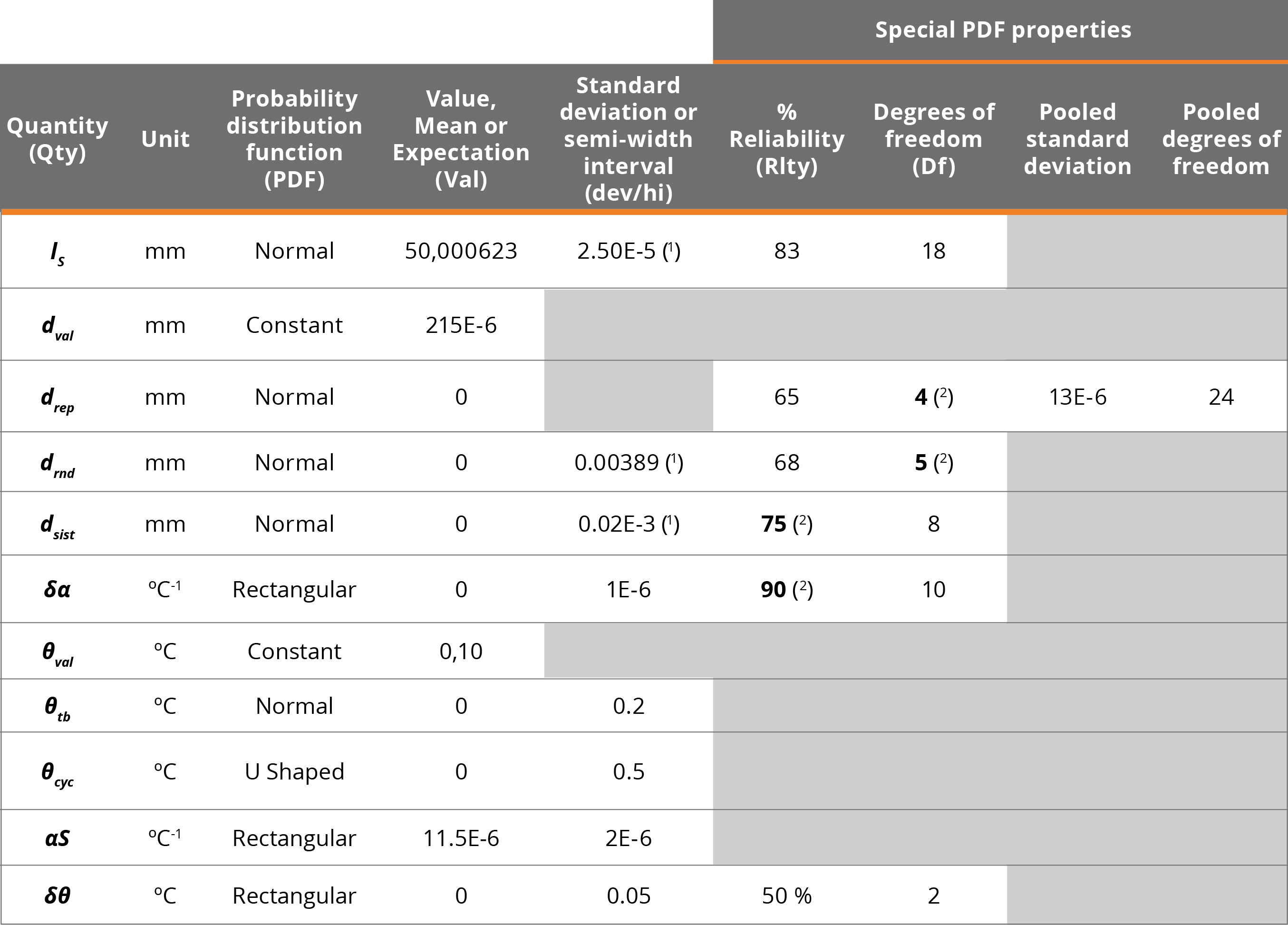
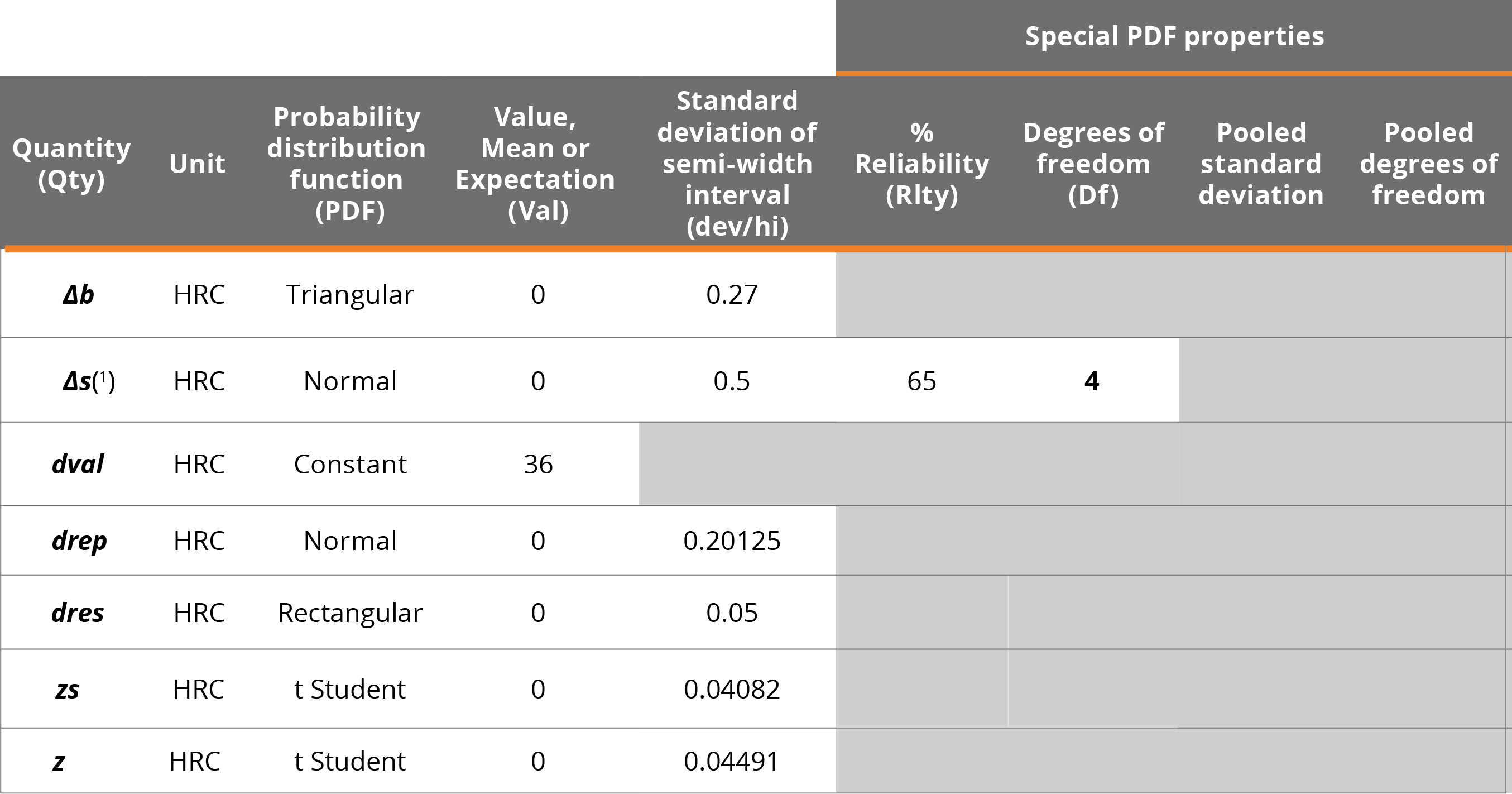
Where Ri represents the relative reliability, as established in MCM Alchimia 5 (Alchimia Project, s.d.). Following Table 1 shows PDF data and calculation that have to be typed in PDF panels of the application.
Table 1. Simulation data of example 1. (1) By selecting “Use calibration certificate”, MCM Alchimia allows to configure a Normal probability distribution, using the expanded uncertainty U and the coverage factor k of a calibration certificate, which is usually better in these cases. The standard deviation indicated in Table 1 is the value resulting from the U/k operation, which the software performs automatically. (2) The values in bold font are taken from the example statement. The software automatically calculates the corresponding reliability or degrees of freedom.
Example 2. Resistance measurement (from: JCGM 100:2008, H2)
Topic: Input of experimental data and use of correlation matrix
This example only considers the evaluation of type A standard uncertainties, based on input variables representing series of observations. In a real case, the existence of systematic effects must also be considered, which are not taken into account in this example. The measurement problem refers to the calculation of the resistance R and the reactance X, from readings of the potential difference between the terminals V, the alternating current I passing through it, and the phase-shift angle between the potential difference and the alternating current. This technical note will only address the measuring of ., since the uncertainty of X and Y can be estimated in the same way.
Directly applying the recommendations of the guide, the experimental data must be input into the mathematical model as variables with t student probability distribution and with degrees of freedom indicated in the example approach. When using a t distribution, it is mandatory to calculate previously the mean and standard deviation of the means as PDF parameters. However, MCM Alchimia (Alchimia Project, s.d.) includes an item called "Experimental" near bottom of the list of probability distributions. This feature allows the technician to input the raw experimental data, from which the application calculates the arithmetic mean, degrees of freedom calculated as n-1 and the standard deviation of the means as s√n , where s is the standard deviation of the sample and n the number of observations. Thus, the random sampling distribution for such a quantity should be student t with means, standard deviation, and degrees of freedom calculated automatically.
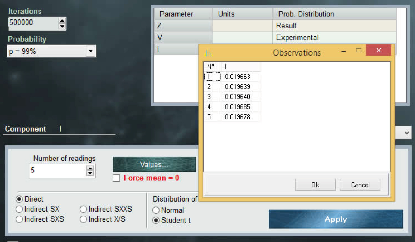
Figure 1. Window for experimental data variables (Experimental PDF).
According to what the example establishes, the input quantities are correlated. The correlations between two random variables (eg x1 and x2) can be calculated previously by determining the covariance from equation 6:

Equation 6
And using the resulting value to determine the correlation coefficient r (x1, x2), according to equation 7:

Equation 7
In equations 6 y 7, s(x̄1,x̄2) represents the covariance of arithmetic means of variables x1, and x2, while x̄1, x̄2, s(x̄1) and s(x̄2) correspond to the arithmetic means of x1 and x2 and their respective standard deviations.
MCM Alchimia (Alchimia Project, s.d.) supports the use of correlated magnitudes in the models, through the window that opens with step 4 button. In this section a correlations matrix is available, with a number of rows and columns equivalent to the magnitudes of which the measurand is function. This matrix is automatically rebuild every time the mathematical model of the trial is modified with a number of rows and columns equal to the number of variables involved in the model. For the estimation of the standard uncertainty of R by the GUM method with correlated input variables, the software calculates numerically, the sensitivity coefficients ci, estimating the standard uncertainty as:

Equation 8
Where UR is the standard uncertainty of measurand R, cv cIand cθ are the sensitivity coefficients of the potential difference, current and phase-shift angle respectively, whereas uV, uI and uθ their respective standard uncertainties. Finally, r(i,j) is the estimated correlation coefficient between the component i and the component j, obtained from equation 9:

Equation 9
Where ui,j is the estimated covariance, associated to V and I.
An interesting approach, not addressed in the JCGM guide, arises when we try to calculate the expanded uncertainty from the standard uncertainty of equation 8 and its effective degrees of freedom. The reference guide indicates that the effective degrees of freedom must be calculated using the Welch-Satterthwite formula.
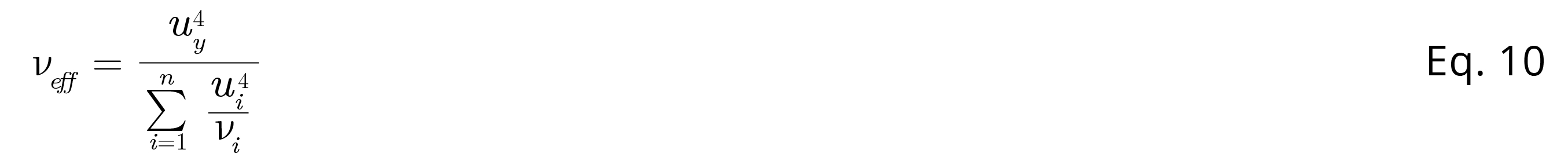
Equation 10
However, an important factor to take into account when calculating the effective degrees of freedom for the modification of the expanded uncertainty, is that the Welch-Sattertwite equation is only valid for models that have independent (uncorrelated) uncertainty components with finite degrees of freedom. Consequently, in this example, the effective degrees of freedom must be calculated by means of an adequate generalization of Welch-Sattertwite formula, to be valid in mathematical models with non-independent error components (Willink, 2007). MCM Alchimia 5 (Alchimia Project, s.d.), implements the generalization of the Welch-Satterthwite formula defined by equation 11 (Castrup, 2010).
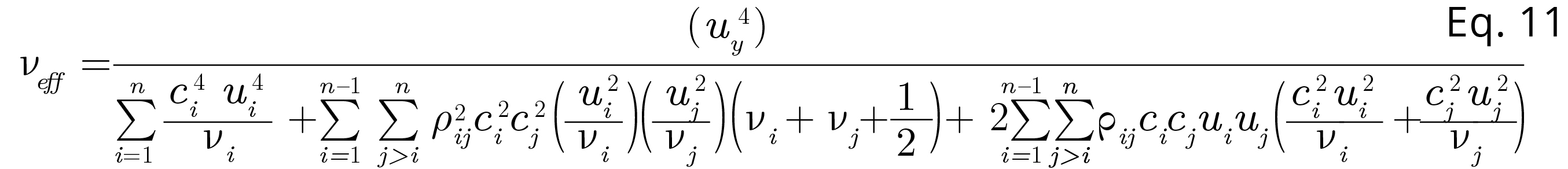
Equation 11
For data processing by the Monte Carlo method, MCM Alchimia (Alchimia Project, s.d.) also supports correlated input quantities. In this case the software carries out the correlation calculations by re-simulating random samples for V and I through a conversion of the correlation matrix indicated in the panel of step 4 into a covariance matrix and then decomposing the latter by means of a Cholesky factorization to obtain a lower triangular matrix. The product of this triangular matrix and the matrix with the uncorrelated input samples is then used to obtain samples with the indicated correlations for the input quantities of the model. The software implements all these operations automatically, so nothing is required to be done, beyond typing the corresponding coefficients in the correlation matrix.
Example 3. Calibration of a thermometer (from: JCGM 100:2008, H3)
Topic: Leasts squares fitting and calibration curves
One of the main tools of MCM Alchimia is the regressions module (Alchimia Project, s.d.). This feature allows the user the user to perform the least squares analysis of a set of values and solve a mathematical model that contains an interpolated value from abscissa or ordinate, as an input variable. The software has two methods for data processing. The first method uses the slope and intercept parameters as input quantity. The secondone uses a specific function to predict a value on one axis from a known value on the other.
Example H.3 of JCGM 100: 2008 (BIPM, et al., 2008a) establishes that both the abscissa and the ordinate in the standard curve are constant values, that is, that their contribution of uncertainty is zero, as well as the temperature of which we want to predict their correction. At this point it is important to note that in most cases of real data this is not true, rather at least the data of the y-axis, either axes or even both, present contributions of uncertainty that, depending on the case, can be significant. This example is solved with the data set out in the reference standard in order to compare results; nevertheless, it is relevant to remember that MCM Alchimia (Alchimia Project, s.d.) supports curves with uncertainties in both axes, one or none. In those cases where uncertainty values are indicated for the axes, the uncertainty contribution of the regression parameters due to stochastic effects are taken into account in the values resulting from the prediction in x-axis or y-axis.
The problem to be addressed is the calibration of a thermometer at 11 points in the range of 21°C to 27°C, comparing the thermometer readings (tk) for which negligible uncertainty is assumed, with the corresponding reference temperature of a calibrated standard (tR,k). Then, the corrections are obtained using a linear regression or the direct square limits method, obtaining slope and intercept parameters.
This example addresses the least squares fitting to obtain the curve and how these slope and intercept parameters, as well as their respective variances and covariances are used to obtain the standard uncertainty limited to the correction, predicted according to equation 12.

Equation 12
The document shows least squares analysis for different abscissa data, varying the value taken for the reference temperature t0. These regression parameters obtained present correlation coefficients of different magnitude according to the set of input values used (that is, for each value of t0). The correlation between the slope and the ordinate at the origin can even be null by taking:

Equation 13
Finally, with the calculated regression coefficients, the correction for t = 30 °C and its standard uncertainty are estimated, obtaining the same result regardless of the value of t0 used.
If we want to reproduce this calculation with MCM Alchimia (Alchimia Project, s.d.), in the same way that the document does, we can use the expression of equation 12 as the mathematical model of the test. Then, to assign probability distributions to the regression coefficients y1 and y2. The software has available a tool in the list of PDF called Regression, where the corresponding curve parameter can be selected without entering any additional information. The software automatically performs the required numerical assignments for based on the data from the connected regression. Of course, the regression parameters are only available for models with a connected curve.
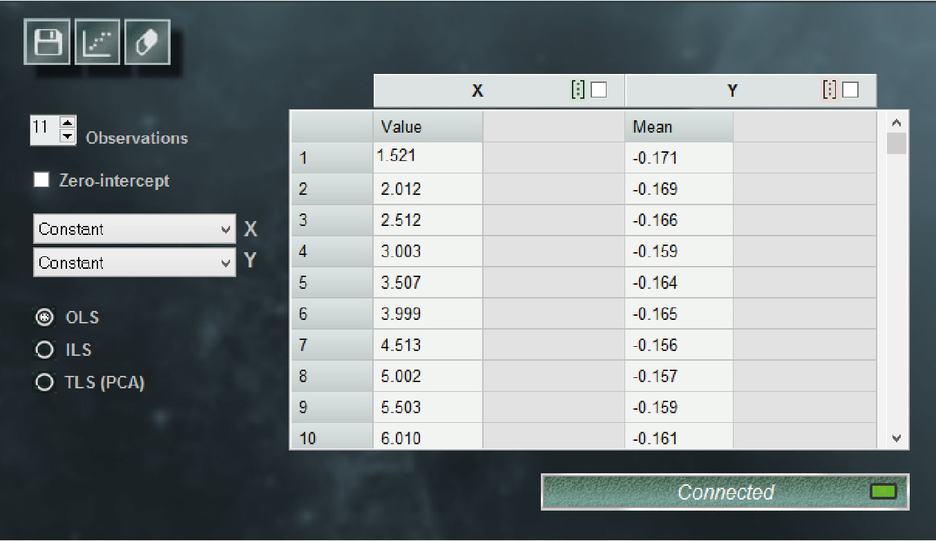
Figure 2. MCM Alchimia regression window (Alchimia Project, s.d.).
According to the text of the reference document, the slope and intercept are correlated. The correlation coefficient can be calculated with equation 14:

Equation 14
Where r, is the correlation coefficient for the ordinate at the origin (intercept) (y1) and the slope (y2), n the number of observations, θk = (tk – t0), with t0 the reference temperature, in this case t0 = 20 °C according to what was stated. Eq. 11 it results in r(y1,y2) = -0.930. This value must be entered into the correlation matrix by clicking on the button of step 4 of the software.
Example 4. Measurement of activity (from: JCGM 100:2008, H4)
Topic: Repeatability
This example consists in the determination of the Radon (222Rn) activity in a water sample by counting the liquid scintillation by comparison with a standard sample of radon in water of known activity. The determination is carried out by measuring the pattern of known activity, a sample of water without radioactive substance and the sample with unknown activity.
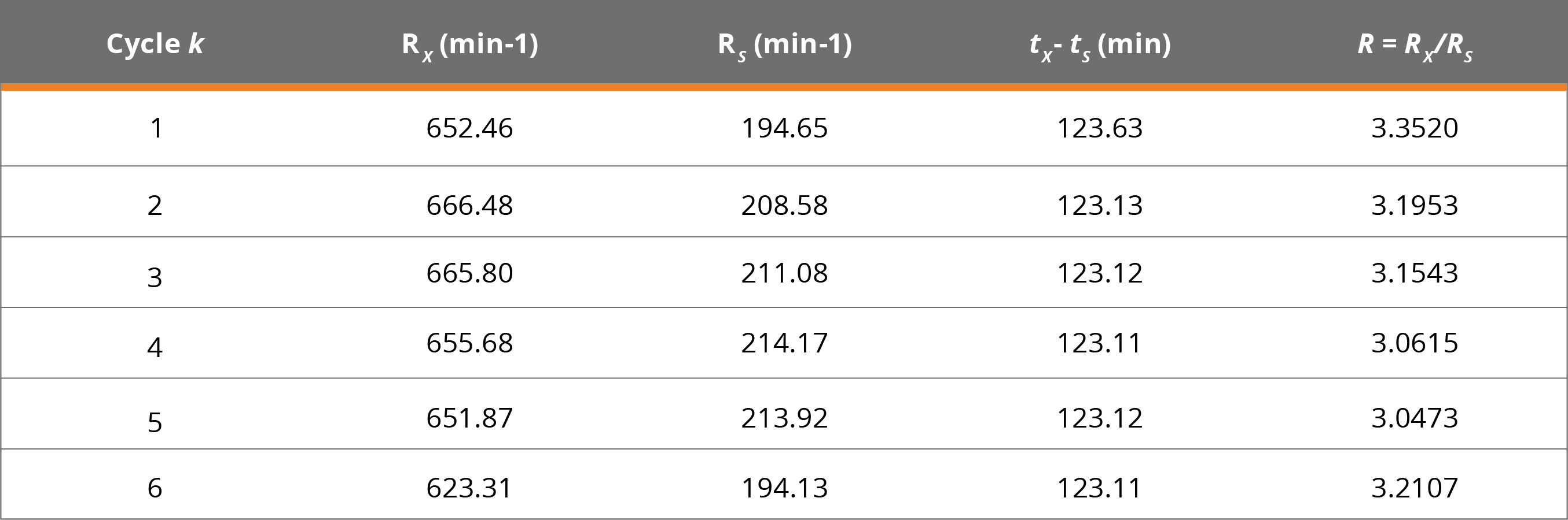
The presentation of the problem shows a table with six measurement cycles from each of the three counting sources, with a counting interval of t0 = 60 min. From this table, the count corrected for background noise Rx and decay Rs are calculated, according to equations 15 and 16:

Equation 15

Equation 16
Obtaining a new table with the following results.
Table 2. Corrected count results for the 6 cycles. With a correlation coefficient between R. and R. : r(R.,R.) = 0.646.
Example 4 presents two ways to solve the problem. Both approaches can be reproduced with MCM Alchimia (Alchimia Project, s.d.). The first way is to use mean values of Rx and Rs, taking into account the correlation between these values. The equation to obtain the known activity Ax will be equation 17:

Equation 17
To solve it using MCM Alchimia (Alchimia Project, s.d.), it is better to assign experimental values to RX and RS instead of a Gaussian or t distribution. This method of using experimental values with the software is explained in Example 2.
Before running the simulation and GUM estimation, it is mandatory to enter the correlation coefficient in the correlation matrix and connect it to the model.
Example 4 of JCGM100: 2008 (BIPM, et al., 2008a), establishes also a second approach to the solution that dispenses with the use of correlated variables, by means of the ratio R = RX / RS, which can be calculated more simply by means of equation 18:

Equation 18
And using the mean of the six values in the equation 19:

Equation 19
Applying these changes to the mathematical model and overriding the correlation, results identical to those of the other method are obtained.
Example 5. Rockwell hardness measurement (from: JCGM 100:2008, H6)
Topic: Standard deviation of the sample mean, without knowing the individual observations
In this case, the example addresses the hardness measurement of a sample block of material, on the Rockwell "C" scale. For this purpose, a measuring machine previously calibrated with a standard machine is used.
The hardness test is carried out by pressing an indenter of specific dimensions, with a defined force, on the surface of the material under test. Hardness can be determined as the arithmetic mean of a given number of indentor penetration depth measurements. The unit of hardness on the Rockwell-C scale is 0.002 mm, with a hardness on that scale defined as 100 × (0.002 mm) minus the average depth measured in mm, of 5 penetrations.
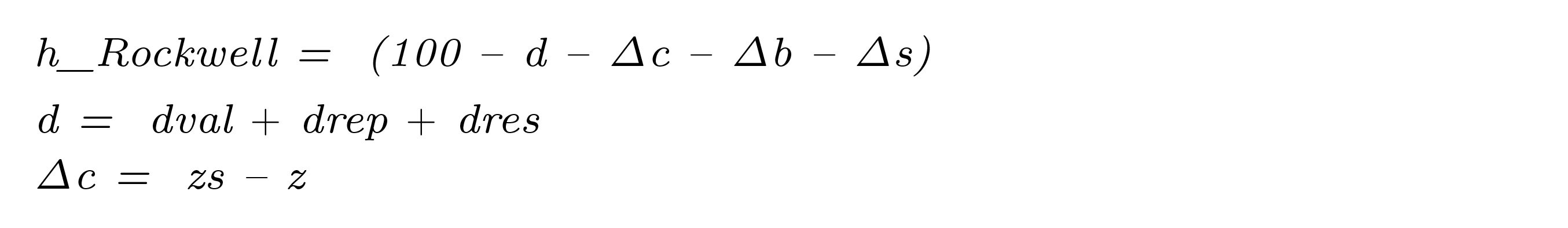
The mathematical model for determining hardness involves not only the average depth of the prints made with the indentor of the calibration machine, but also the average depth of indentations made in the same block by the master machine. Thus, the mathematical model can be presented in mm, as:

Equation 20
Where d̅ is the average depth of five penetrations made with the calibration machine, Δc is the correction obtained from a comparison between the calibration machine and the standard machine. Δb is the difference in hardness between two areas of the transfer block surface tested by the two machines, and Δs the uncertainty contribution of the pattern machine. The suffix mm in the variables indicates that they must be in this unit in this equation.
Since the data is given in units of the Rockwell scale we can rewrite the equation in these units:

Equation 21
In equations 20 and 21, the quantity d̅ has two components of uncertainty, due to the repetition of observations and the other due to the indication or resolution of the equipment. As in example 1, the random variable is split into value and uncertainty components:

Equation 22
Where dval is the arithmetic mean of depth measurements, dres the uncertainty contribution due to resolution and drep the repeatability component. In this equation, dval it is a constant of value 36.0 Rockwell scale units. drep corresponds to a type A uncertainty component. The example statement indicates a sample standard deviation of 0.45 units, however, it is necessary to take into account that the variable d corresponds to an average of five values. Therefore, the uncertainty component must be the standard deviation of the sample means, that is, divide the given value of the sample standard deviation by the square root of the number of observations in the sample.
Thus, u(drep) = 0.45/ √5 = 0.20125. The distribution function to be assigned can be a t-distribution with 4 degrees of freedom. If you want to use a normal distribution, it is also possible and you will get identical results although in this case you must also assign 4 degrees of freedom in the advanced configuration panel of the normal distribution.
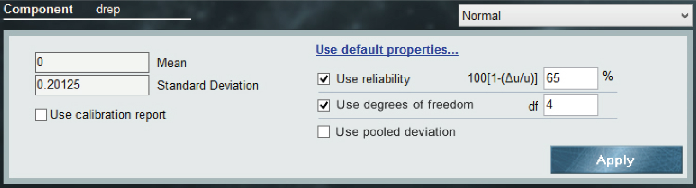
Figure 3
Figure 3. Advanced configuration of the Normal (Gaussian) distribution.
The correction of the calibration machine with respect to the standard machine, Δc, can also be split into two terms, the mean of the experimental variance of the standard machine zs, from the measuring machine, z, so Δc can be rewritten:

Equation 23
For the variables zs and z, the square root of the experimental variance is given, of 0.10 units and 0.11 units respectively. Applying the same method as for drep in both cases the number of observations is 6, therefore the degrees of freedom will be 5 for the two variables, in a t distribution with a value of 0 and standard deviation 0.10/√5 = 0.04082 and 0.11/√5 = 0.04491 for zs y z respectively.
For the final model, then it can be typed in the MCM Alchimia (Alchimia Project, s.d.), equation set field:
Next, the probability distribution set is configured:
Table 3. Simulation data of example 5. (1) This input quantity was configured with a Normal distribution including degrees of freedom data from the advanced settings panel. However, it is possible to assign a t distribution with the same standard deviation and degrees of freedom, obtaining identical results.
Example 6. Additive mathematical model (from: JCGM 101:2008, 9.2)
Topic: Validation of GUM results with MCM
Supplement 1 to the guide addresses the use of the Monte Carlo method when Mathematical Models make the application of GUM difficult. However, it is possible to solve them by both methods with the use of MCM Alchimia (Alchimia Project, s.d.). This example shows a simple case where the impact of the real distribution of the measurand obtained by MCM on the coverage interval and the departure from the coverage interval obtained for the same probability can be seen, by means of the approximation to a normal distribution applying the GUM method. The measuring problem is a sum of 4 terms in three different sets of PDF:

Equation 24
Case 1: Xi Gaussian PDF of mean = 0 and standard deviation = 1
Case 2: Xi Rectangular PDF of mean = 0 and semi-width interval = 1
Case 3: same as case 2 but with X4 rectangular of mean = 0 and semi-width 10
In all cases, the numerical tolerance of the expanded uncertainty and the difference between the values obtained by GUM and MCM are studied to assess whether the GUM method can be considered adequate for the model or validated by MCM.
Example 7. Mass calibration (from: JCGM 101:2008, 9.3)
Topic: Complex mathematical models
This example refers to the calibration of a weight W by comparison with a reference weight R. The mathematical model of the test is determined by the following equation:

Equation 25
Where δm the deviation of the mass of the sample weight W with respect to the nominal value, mR,c the mass of the standard weight, δmR,c the difference in mass between W and R, ρathe air density during the test. ρa0 = 1.2 kg/m3, is the air density in the definition of conventional mass, ρw and ρR density of weight W and weight R respectively.
The objective of the treatment in this example is to show the greater ease offered by the MCM method compared to the GUM approach, due to the mathematical complexity of the model and the avoidance of individual symbolic derivation of the input quantities with respect to the measurand function. The use of MCM Alchimia (Alchimia Project, s.d.), makes obtaining a classic GUM uncertainty budget simple, without requiring either knowing the partial derivatives in the model. It is necessary to note that the software does not perform symbolic derivation, for the input quantities, rather they are calculated by numerical approximation, according to the Kragten method (Kragten, 1995). Assuming that the standard uncertainties of the input quantities are much less than their value, the sensitivity coefficients (partial derivatives) can be obtained by approximation to the tangent value of the measurand function:

Equation 26
According to the established in the example, the equation to type in the software can be:
δm = (m_Rc + δm_Rc)*(1+(ρa-ρa0)*(1/ρW+1/ρR))-m_nom
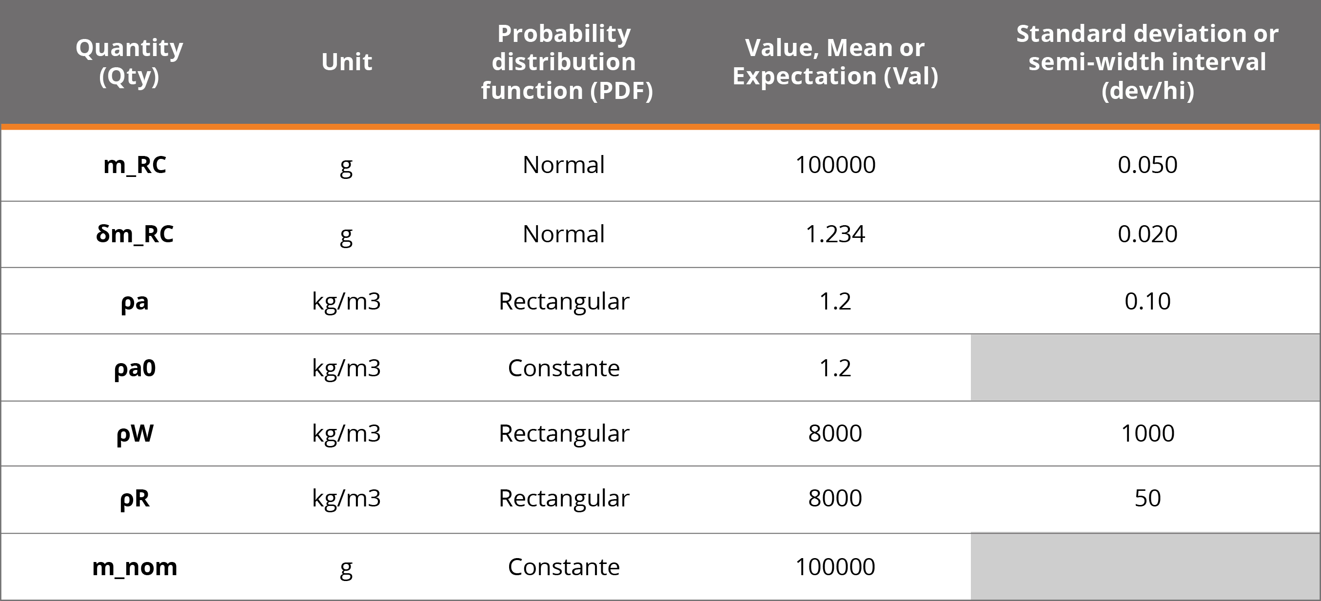
The set of values to configure the PDFs are detailed in Table 4.
Table 4. Example 7 simulation data.
RESULTS AND DISCUSSION
Example 1. Calibration of end gauge blocks. After running the simulation for a 99% coverage probability, the following results are obtained according to GUM and MCM.
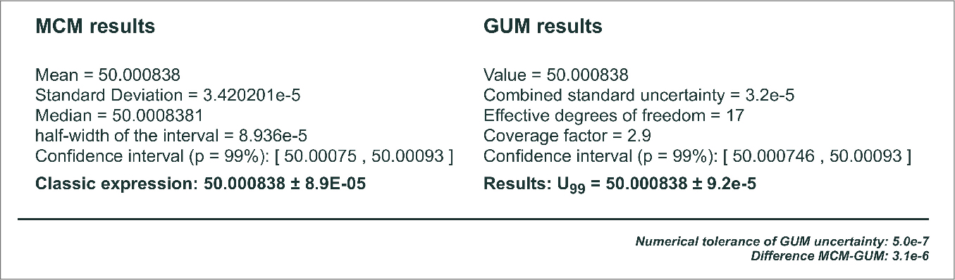
Figure 4. Summary results of GUM and MCM for Example 1.
As expected, the results are close to those shown by the reference document, except for small differences due to rounding. It is observed that the results obtained by Monte Carlo are identical to those obtained when the GUM method is applied including higher order terms in the Taylor series approximation, JCGM 100:2008 H.1.7 (BIPM, et al., 2008a).
Example 2. Resistance measurement. For this example, the following results are found for resistance R according to the GUM and MCM approaches:
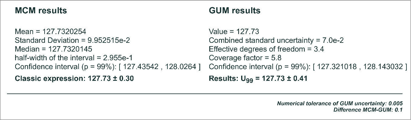
Figure 5. Summary results for example 2.
The results obtained for uR are equivalent to those indicated in table H.3 of the guide. At this point it should be noted that there are significant differences between the results obtained by both methods for the expanded uncertainty value.
This is mainly due to the form of the probability distribution function presented by the Monte Carlo random sample. Since the distribution of the measurand departs from a Normal or t distribution, the uncertainties obtained by GUM differ from those obtained by MCM. In these cases, the standard uncertainty calculated according to the GUM approach is no longer a reliable representation of the actual uncertainty. Figure 6 shows the resulting functions for GUM and MCM, where the difference between the curves can be seen.
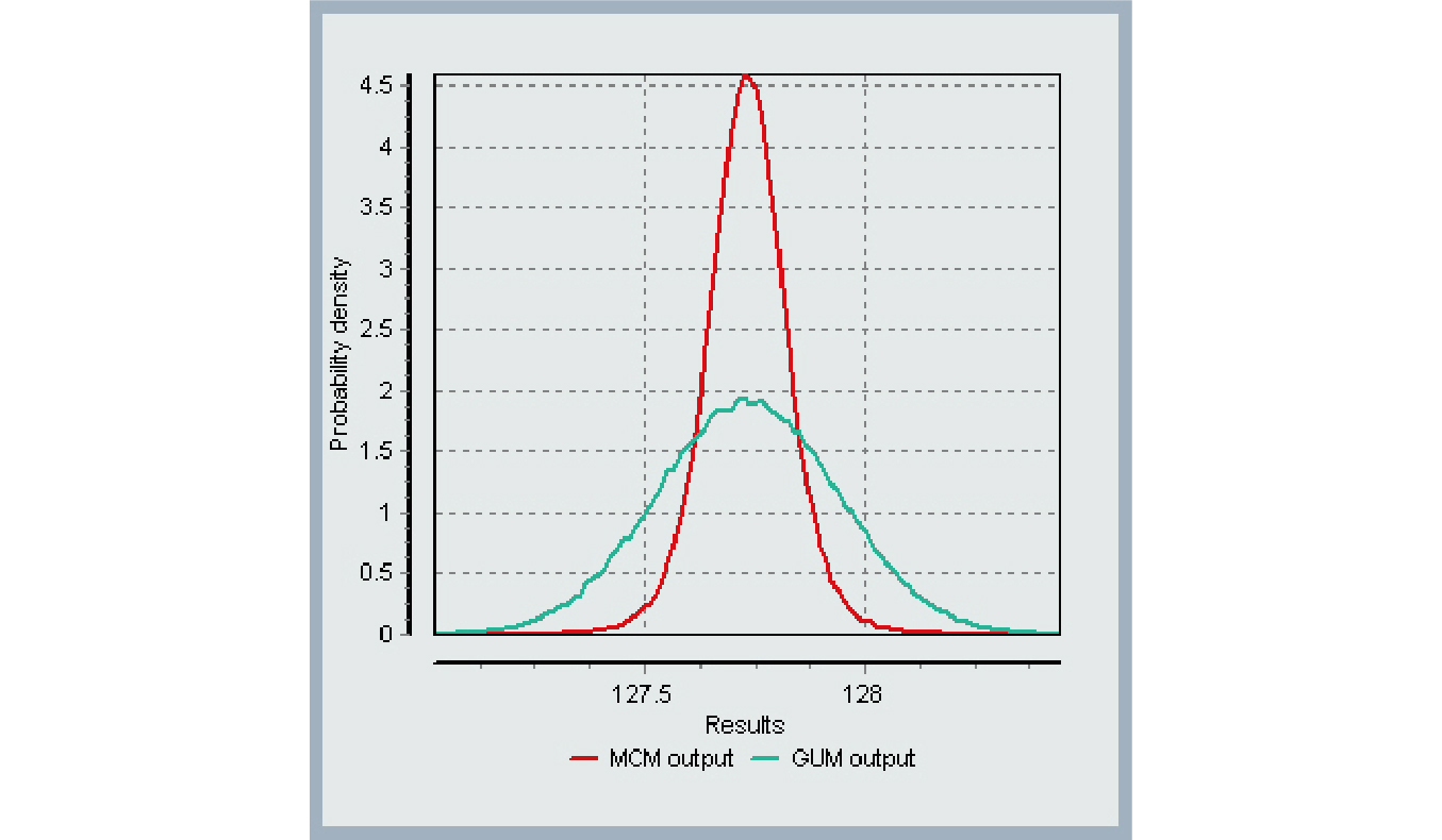
Figure 6. Graph with the resulting GUM and MCM curves.
Example 3. Calibration of a thermometer. This example was solved in the same way as the reference document by using correlated variables, obtaining the following results for R.
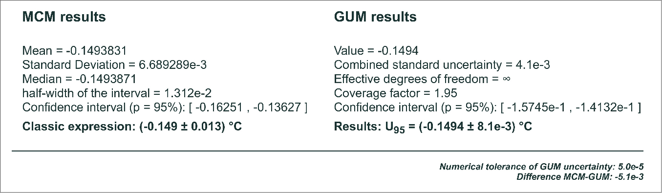
Figure 7. Results of Example 3 for the mathematical model using regression parameters.
A different approach to the solution. The previous development has the difficulty of the mandatory using of r (y1,y2) or, otherwise, it has to be redo the least-squares fitting after shifting the x-axis to a value for which the covariance between the regression parameters is null (eg choosing a value of t0 = 24.0085 in this example). There is, however, an available feature in MCM Alchimia (Alchimia Project, s.d.), for models with calibration curves prediction, that dispense with the correction due to correlations. This approach involves using two functions: Reg_y(x) to predict a value in ordinates (y) from a known value on the x-axis; and Reg_x(y) similar to the previous one but exchanging axes, that is, to predict a value of the independent variable (x-axis) from a value of the dependent variable (y-axis). The latter case is common in analytical chemistry measurements, for example, to determine the concentration of a sample from its absorbance value, by means of a previously established calibration or standard curve. The calibration curve should show the concentration in abscissa and the absorbance in ordinate.
The mathematical model to type in the field of software equations, after connecting the curve, will then be:
Corr = REG_Y(tk-tr), where tk is the temperature to predict its correction and tr the reference temperature.
This is the recommended method to deal with mathematical model of measurements involving least squares analysis. Finally, the results obtained by this method are identical to those calculated using regression parameters, with the advantage of dispensing with the study of correlations or other lateral calculations.
Example 4. Measurement of activity. The results obtained with MCM Alchimia (Alchimia Project, s.d.), for AX according to the GUM and Monte Carlo methods are shown in the following graph. This result is identical in both presented solution approaches.
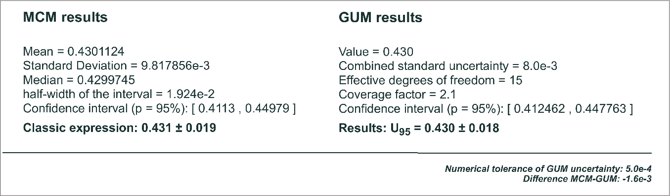
Figure 8. Summary of results from Example 4.
Example 5. Rockwell hardness measurement. The results obtained in this example are summarized in the following figure.
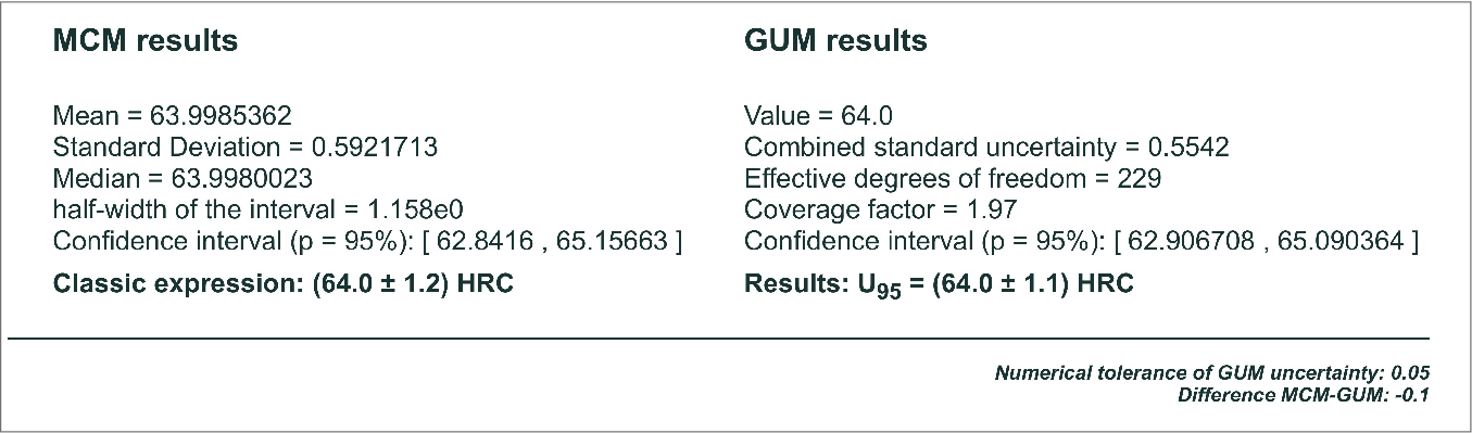
Figure 9. Summary of results from Example 5.
Example 6. Additive mathematical model. The results obtained for the three sets of distributions are shown in the following table, expressed as half-width of the coverage interval, equivalent to the expanded uncertainty, although expressed with more significant digits to enable the comparison between both methods:
Table 5. Results for three sets of distributions.
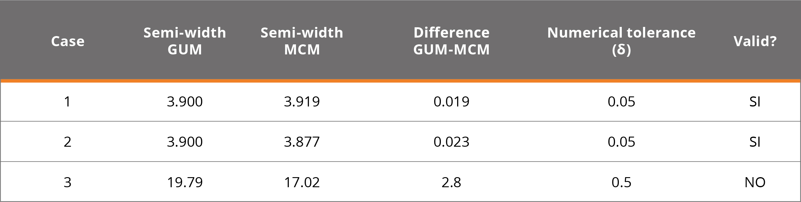
In the third case, it does not comply with the validation of GUM by MCM, because the largest contributor of the uncertainty is rectangular, resulting in a departure from the application conditions of the Central Limit Theorem. In those cases, the GUM approach is not precise obtaining a uncertainty value. The following figure shows the graphs of the results for the three cases where you can see the difference between models 1 and 2 that met the validation and 3 that did not.
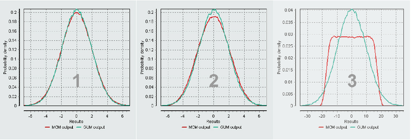
Figure 10. Chart of results of GUM and MCM for 3 cases.
Example 7. Mass calibration. The following figure shows the results window of the program for the Monte Carlo method. It can be seen that the result is identical to that obtained in the reference document.
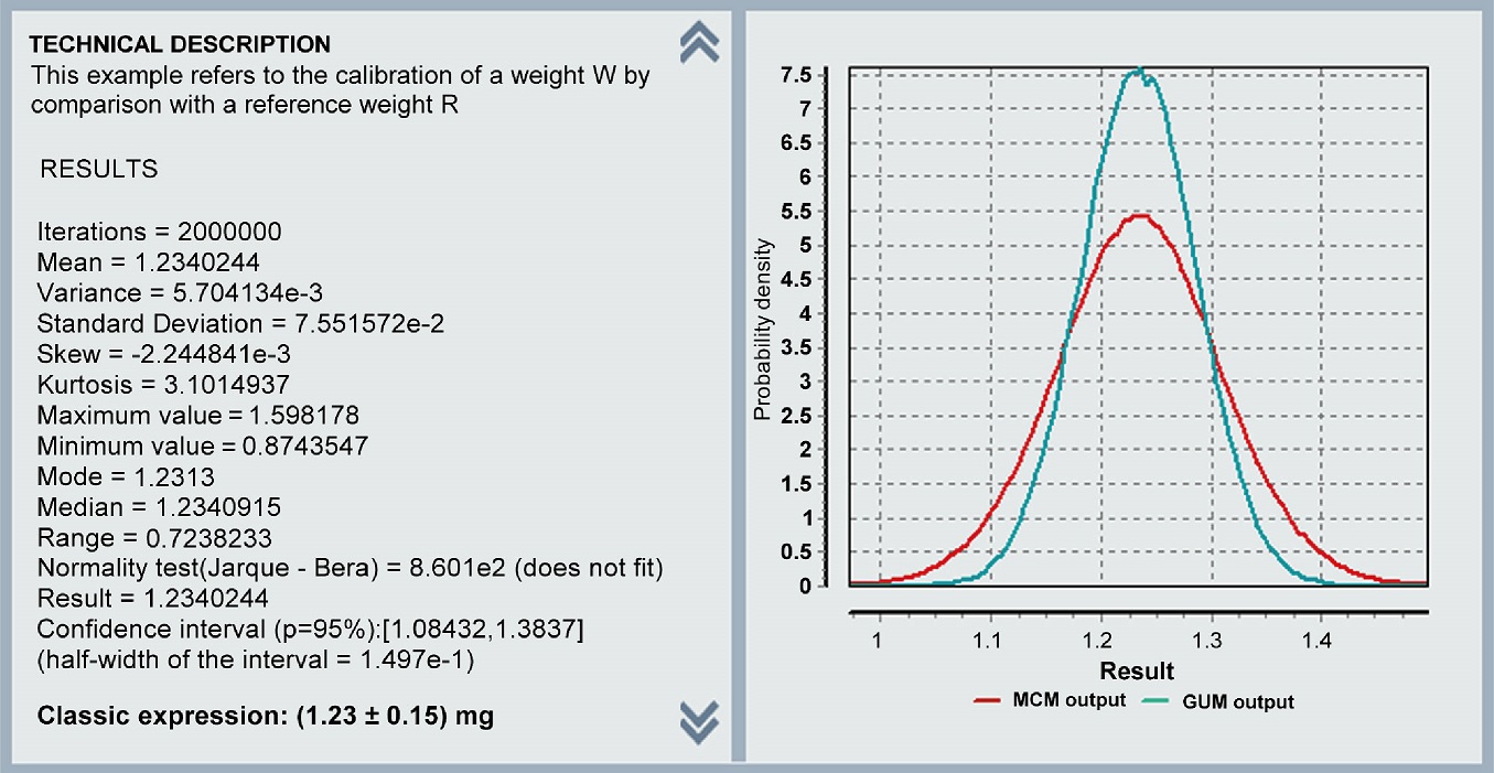
Figure 11. MCM Alchimia results window for example 7 (Alchimia Project, s.d.).
The data on the left side, shows the statistical data of the simulated random sample and on the right side is plotted the real distribution obtained by the simulation, and the normal distribution of the GUM method with first-order terms. The difference between the two curves explains the differences between the uncertainty results for both approaches.
*The complete calculation models por MCM Alchimia used in the examples in this technical note can be viewed at the link:
https://ojs.latu.org.uy/index.php/INNOTEC/article/view/547
CONCLUSIONS
Although there are a large number of software applications available for estimating uncertainties, the treatment of measurements in real tests often has characteristics that make it difficult to process them by these applications, for example, assigning reliability percentages to uncertainties type B, interpolation in calibration curves, simulation of regression coefficients, application of the Monte Carlo method to correlated variables, etc.
The examples in the JCGM 100: 2008 (BIPM, et al., 2008a) and JCGM 101: 2008 (BIPM, et al., 2008b) reference guides present many of these aspects which are addressed in this technical note. This work shows that the MCM Alchimia software (Alchimia Project, s.d.) implements many features that make it able to deal with special situations or complex mathematical models in a simple way. Methods detailed here not only used to ease the process, but also to reduce the possibility of errors that are commonly inadvertent in uncertainty quantification, for example, the non-consideration of correlation between regression coefficients, or use basic Welch-Satterthwite formula in order to calculate effective degrees of freedom with non-independent quantities.
Moreover, MCM Alchimia (Alchimia Project, s.d.), puts at disposal unusual relevant information for example, the comparison of confidence intervals by GUM and MCM in the summary of results, which allows validation of the classic calculations according to JCGM 101: 2008 (BIPM, et al., 2008b) without requiring any side calculation, or the complete simulated sample for external worksheet treatment or analysis.
Finally, all the obtained outcomes using the software are identical or very close to those indicated in the reference documents. Therefore, although it is necessary to carry out additional tests to consider MCM Alchimia (Alchimia Project, s.d.), fully validated, these examples represent a form of validation of the software for the topics and features discussed.
REFERENCES
Alchimia Project, s.d. MCM Alchimia, MCM & GUM uncertainty estimation engine [On line]. Version 5. [s.l.]: Alchimia Project. [Accessed: June 15, 2020] Available at: http://www.mcm-alchimia.com
BIPM, IEC, IFCC, ILAC, ISO, IUPAC, IUPAP and OIML, 2008a. JCGM 100:2008 GUM 1995 with minor corrections. Evaluation of measurement data — Guide to the expression of uncertainty in measurement. [s.l.]: JCGM.
BIPM, IEC, IFCC, ILAC, ISO, IUPAC, IUPAP and OIML, 2008b. JCGM 101:2008 Evaluación of measurement data – Supplement 1 to the Guide to the expression of uncertainty in measurement – Propagation of distributions using a Monte Carlo method. [s.l.]: JCGM
BIPM, IEC, IFCC, ILAC, ISO, IUPAC, IUPAP and OIML, 2012. JCGM 200:2021 International vocabulary of metrology – Basic and general concepts and associated terms (VIM). [s.l.]: JCGM
Castrup, H., 2010. A welch-satterthwaite relation for correlated errors [On line]. In: Meas. Sci. Conf., Pasadena. [Accessed: April 16, 2020]. Available at: https://www.semanticscholar.org/paper/A-Welch-Satterthwaite-Relation-for-Correlated-1-Castrup/7c9a41aa3cce0bb79e69bc820369c4e2ec1a7e3c
Constantino, P., 2013. Computational aspects in uncertainty estimation by Monte Carlo Method [On line]. In: INNOTEC, 8, pp.13-22. [Accessed: April 16, 2020]. Available at: https://ojs.latu.org.uy/index.php/INNOTEC/article/view/214
Kragten, J., 1995. A standard scheme for calculating numerically standard deviation and confidence intervals. In: Chemometrics and Intelligent Laboratory Systems, 28(1), pp.89-97. DOI: https://doi.org/10.1016/0169-7439(95)80042-8
Santana, M. and Kalid, R., 2019. Fundamentos estadísticos para la evaluación de la incertidumbre en las calibraciones [On line]. In: CENAM. Workshop on Statistic, Data Analysis and Measurement Uncertainty for Meteorology. Querétaro, México (02 de diciembre de 2019. Querétaro: CENAM. [Accessed: April 16, 2020]. Available at: https://zenodo.org/record/4021356#.YBzRXKdKjDd. http://doi.org/10.5281/zenodo.4021356
Willink, R., 2007. A generalization of the Welch–Satterthwaite formula for use with correlated uncertainty components. In: Metrologia, 44(5), pp.340.